The Gaussian distribution
The default probability distribution
June 27, 2016 — July 19, 2023
Many facts about the useful, boring, ubiquitous Gaussian. Djalil Chafaï lists Three reasons for Gaussians, emphasising more abstract, not-necessarily generative reasons.
- Gaussians as isotropic distributions — a Gaussian is the only distribution that can be both marginally independent and isotropic.
- Entropy maximizing (the Gaussian has the highest entropy out of any distribution wath fixed variance and finite entropy)
- The only stable distribution with finite variance
Many other things give rise to Gaussians; sampling distributions for test statistics, bootstrap samples, low dimensional projections, anything with the right Stein-type symmetries, central limit threorems… There are many post hoc rationalisations that use the Gaussian in the hope that it is close enough to the real distribution: such as when we assume something is a Gaussian process because they are tractable, or seek a noise distribution that will justify quadratic loss, when we use Brownian motions in stochastic calculus because it comes out neatly, and so on.
1 Density, CDF
1.1 Moments form
The standard (univariate) Gaussian pdf is \[ \psi:x\mapsto \frac{1}{\sqrt{2\pi}}\text{exp}\left(-\frac{x^2}{2}\right). \] Typically we allow a scale-location parameterised version \[ \phi(x; \mu,\sigma ^{2})={\frac {1}{\sqrt {2\pi \sigma ^{2}}}}e^{-{\frac {(x-\mu )^{2}}{2\sigma ^{2}}}} \] We call the CDF \[ \Psi:x\mapsto \int_{-\infty}^x\psi(t) dt. \] In the multivariate case, where the covariance \(\Sigma\) is strictly positive definite, we can write a density of the general normal distribution over \(\mathbb{R}^k\) as \[ \psi({x}; \mu, \Sigma) = (2\pi )^{-{\frac {k}{2}}}\det(\Sigma)^{-\frac{1}{2}}\,\exp ({-\frac{1}{2}( x-\mu)^{\top}\Sigma^{-1}( x-\mu)}) \] If a random variable \(Y\) has a Gaussian distribution with parameters \(\mu, \Sigma\), we write \[Y \sim \mathcal{N}(\mu, \Sigma)\]
1.2 Canonical form
Hereafter we assume that we are talking about multivariate Gaussians,. or this is not very interesting. Davison and Ortiz (2019) recommends the “information parameterization” of Eustice, Singh, and Leonard (2006), which looks like the canonical form to me. \[ p\left(\mathbf{x}\right)\propto e^{\left[-\frac{1}{2} \mathbf{x}^{\top} \Lambda \mathbf{x}+\boldsymbol{\eta}^{\top} \mathbf{x}\right]} \] The parameters of the canonical form \(\boldsymbol{\eta}, \Lambda\) relate to the moments via \[\begin{aligned} \boldsymbol{\eta}&=\Lambda \boldsymbol{\mu}\\ \Lambda&=\Sigma^{-1} \end{aligned}\] The information form is convenient as multiplication of distributions (when we update) is handled simply by adding the information vectors and precision matrices — see Marginals and conditionals.
1.3 Annealed
Call the \(\alpha\)-annealing of a density \(f\) the density \(f^\alpha\) for \(\alpha\in(0,1]\). Are there any simplications we can get to evaluate this, e.g. for special values of \(\alpha\)? TBC.
2 Fun density facts
Sometimes we do stunts with a Gaussian density.
2.1 What is Erf again?
This erf, or error function, is a rebranding and reparameterisation of the standard univariate normal cdf. It is popular in computer science, AFAICT because calling something an “error function” is provides an amusing ambiguity to pair with the one where we are used to with the “normal” distribution. There are scaling factors tacked on.
\[ \operatorname{erf}(x) = \frac{1}{\sqrt{\pi}} \int_{-x}^x e^{-t^2} \, dt \] which is to say \[\begin{aligned} \Phi(x) &={\frac {1}{2}}\left[1+\operatorname{erf} \left({\frac {x}{\sqrt {2}}}\right)\right]\\ \operatorname{erf}(x) &=2\Phi (\sqrt{2}x)-1\\ \end{aligned}\]
2.2 Taylor expansion of \(e^{-x^2/2}\)
\[ e^{-x^2/2} = \sum_{k=0}^{\infty} (2^(-k) (-x^2)^k)/(k!). \]
2.3 Score
\[\begin{aligned} \nabla_{x}\log\psi({x}; \mu, \Sigma) &= \nabla_{x}\left(-\frac{1}{2}( x-\mu)^{\top}\Sigma^{-1}( x-\mu) \right)\\ &= -( x-\mu)^{\top}\Sigma^{-1} \end{aligned}\]
3 Differential representations
First, trivially, \(\phi'(x)=-\frac{e^{-\frac{x^2}{2}} x}{\sqrt{2 \pi }}.\)
3.1 Stein’s lemma
Meckes (2009) explains Stein (1972)’s characterisation:
The normal distribution is the unique probability measure \(\mu\) for which \[ \int\left[f^{\prime}(x)-x f(x)\right] \mu(d x)=0 \] for all \(f\) for which the left-hand side exists and is finite.
This is incredibly useful in probability approximation by Gaussians where it justifies Stein’s method.
3.2 ODE representation for the univariate density
\[\begin{aligned} \sigma ^2 \phi'(x)+\phi(x) (x-\mu )&=0, \text{ i.e.}\\ L(x) &=(\sigma^2 D+x-\mu)\\ \end{aligned}\]
With initial conditions
\[\begin{aligned} \phi(0) &=\frac{e^{-\mu ^2/(2\sigma ^2)}}{\sqrt{2 \sigma^2\pi } }\\ \phi'(0) &=0 \end{aligned}\]
🏗 note where I learned this.
3.3 ODE representation for the univariate icdf
From (Steinbrecher and Shaw 2008) via Wikipedia.
Write \(w:=\Psi^{-1}\) to keep notation clear. It holds that \[ {\frac {d^{2}w}{dp^{2}}} =w\left({\frac {dw}{dp}}\right)^{2}. \] Using initial conditions \[\begin{aligned} w\left(1/2\right)&=0,\\ w'\left(1/2\right)&={\sqrt {2\pi }}. \end{aligned}\] we generate the icdf.
3.4 Density PDE representation as a diffusion equation
Z. I. Botev, Grotowski, and Kroese (2010) notes
\[\begin{aligned} \frac{\partial}{\partial t}\phi(x;t) &=\frac{1}{2}\frac{\partial^2}{\partial x^2}\phi(x;t)\\ \phi(x;0)&=\delta(x-\mu) \end{aligned}\]
Look, it’s the diffusion equation of Wiener process. Surprise! If you think about this for a while you end up discovering Feynman-Kac formulae.
3.5 Roughness of the density
Univariate —
\[\begin{aligned} \left\| \frac{d}{dx}\phi_\sigma \right\|_2 &= \frac{1}{4\sqrt{\pi}\sigma^3}\\ \left\| \left(\frac{d}{dx}\right)^n \phi_\sigma \right\|_2 &= \frac{\prod_{i<n}2n-1}{2^{n+1}\sqrt{\pi}\sigma^{2n+1}} \end{aligned}\]
4 Tails
For small \(p\), the quantile function has the asymptotic expansion \[ \Phi^{-1}(p) = -\sqrt{\ln\frac{1}{p^2} - \ln\ln\frac{1}{p^2} - \ln(2\pi)} + \mathcal{o}(1). \]
4.1 Mills ratio
Mills’ ratio is \((1 - \Phi(x))/\phi(x)\) and is a workhorse for tail inequalities for Gaussians. See the review and extensions of classic results in Dümbgen (2010), found via Mike Spivey. Check out his extended justification for the classic identity
\[ \int_x^{\infty} \frac{1}{\sqrt{2\pi}} e^{-t^2/2} dt \leq \int_x^{\infty} \frac{t}{x} \frac{1}{\sqrt{2\pi}} e^{-t^2/2} dt = \frac{e^{-x^2/2}}{x\sqrt{2\pi}}.\]
5 Orthogonal basis
Polynomial basis? You want the Hermite polynomials.
6 Rational function approximations
🏗
7 Entropy
The normal distribution is the least “surprising” distribution in the sense that out of all distributions with a given mean and variance the Gaussian has the maximum entropy. Or maybe that is the most surprising, depending on your definition.
8 Marginals and conditionals
Linear transforms of mutlidimensional Gaussians are especially convenient. You could say that this is a definitive property of the Gaussian. Because we have learned to represent so many things by linear algebra, this means the pairing with Gaussians is a natural one. As made famous by Gaussian process regression in Bayesian nonparametrics.
See, e.g. these lectures, or Michael I. Jordan’s Gaussian backgrounder.
In practice I look up my favourite useful Gaussian identities in Petersen and Pedersen (2012) and so does everyone else I know. You can get a good workout in this stuff especially doing Gaussian belief propagation.
Key trick: we can switch between moment and canonical parameterizations of Gaussians to make it more convenient to do one or the other.

We write this sometimes as \(\mathcal{N}^{-1}\), i.e. \[p(\boldsymbol{\alpha}, \boldsymbol{\beta})=\mathcal{N}\left(\left[\begin{array}{c}\boldsymbol{\mu}_\alpha \\ \boldsymbol{\mu}_\beta\end{array}\right],\left[\begin{array}{cc}\Sigma_{\alpha \alpha} & \Sigma_{\alpha \beta} \\ \Sigma_{\beta \alpha} & \Sigma_{\beta \beta}\end{array}\right]\right)=\mathcal{N}^{-1}\left(\left[\begin{array}{l}\boldsymbol{\eta}_\alpha \\ \boldsymbol{\eta}_\beta\end{array}\right],\left[\begin{array}{ll}\Lambda_{\alpha \alpha} & \Lambda_{\alpha \beta} \\ \Lambda_{\beta \alpha} & \Lambda_{\beta \beta}\end{array}\right]\right)\]
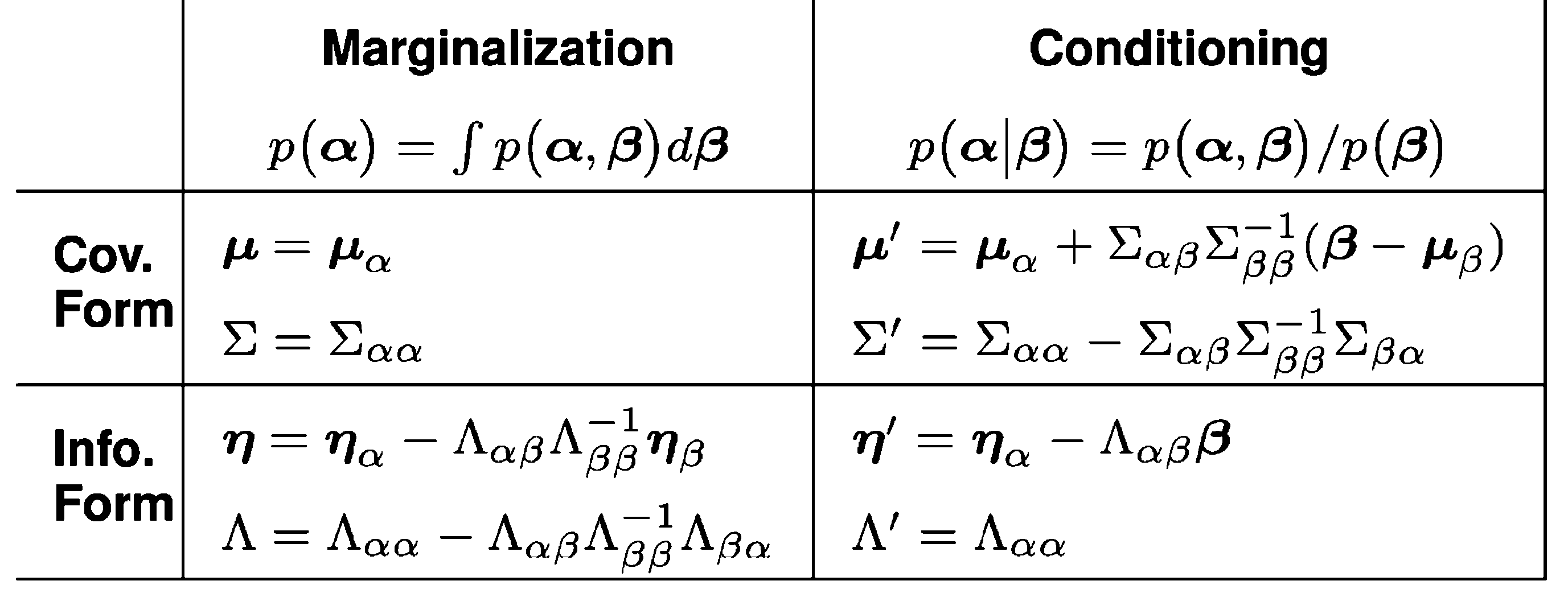
The explicit form the for the marginalising and conditioning ops from Eustice, Singh, and Leonard (2006). I tried to make this table into a real HTML table, but that ends up being a typographical nightmare, so this is an image. Sorry.
Looking at the table with the exact formulation of the update for each RV, we see that the marginalization and conditioning operations are the twins to each other, in the sense that they are the same operation, but with the roles of the two variables swapped.
In GBP we want not just conditioning but a generalisation, where we can find general product densities cheaply.
8.1 Product of densities
A workhorse of Bayesian statistics is the product of densities, and it comes out in an occasionally-useful form for Gaussians.
Let \(\mathcal{N}_{\mathbf{x}}(\boldsymbol{\mu}, \boldsymbol{\Sigma})\) denote a density of \(\mathbf{x}\), then \[ \mathcal{N}_{\mathbf{x}}\left(\boldsymbol{\mu}_1, \boldsymbol{\Sigma}_1\right) \cdot \mathcal{N}_{\mathbf{x}}\left(\boldsymbol{\mu}_2, \boldsymbol{\Sigma}_2\right)\propto \mathcal{N}_{\mathbf{x}}\left(\boldsymbol{\mu}_c, \boldsymbol{\Sigma}_c\right) \] where \[ \begin{aligned} \boldsymbol{\Sigma}_c&=\left(\boldsymbol{\Sigma}_1^{-1}+\boldsymbol{\Sigma}_2^{-1}\right)^{-1}\\ \boldsymbol{\mu}_c&=\boldsymbol{\Sigma}_c\left(\boldsymbol{\Sigma}_1^{-1} \boldsymbol{\mu}_1+\boldsymbol{\Sigma}_2^{-1} \boldsymbol{\mu}_2\right). \end{aligned} \]
Translating that to canonical form, with \(\mathcal{N}^{-1}_{\mathbf{x}}(\boldsymbol{\eta}, \boldsymbol{\Sigma})\) denoting a canonical-form density of \(\mathbf{x}\), then \[ \mathcal{N}_{\mathbf{x}}^{-1}\left(\boldsymbol{\eta}_1, \boldsymbol{\Lambda}_1\right) \cdot \mathcal{N}_{\mathbf{x}}^{-1}\left(\boldsymbol{\eta}_2, \boldsymbol{\Lambda}_2\right)\propto \mathcal{N}_{\mathbf{x}}^{-1}\left(\boldsymbol{\eta}_c, \boldsymbol{\Lambda}_c\right) \] where \[ \begin{aligned} \boldsymbol{\Lambda}_c&=\boldsymbol{\Lambda}_1+\boldsymbol{\Lambda}_2 \\ \boldsymbol{\eta}_c&=\boldsymbol{\eta}_1+ \boldsymbol{\eta}_2. \end{aligned} \]
8.2 Orthogonality of conditionals
See pathwise GP.
9 Fourier representation
The Fourier transform/Characteristic function of a Gaussian is still Gaussian.
\[\mathbb{E}\exp (i\mathbf{t}\cdot \mathbf {X}) =\exp \left( i\mathbf {t} ^{\top}{\boldsymbol {\mu }}-{\tfrac {1}{2}}\mathbf {t} ^{\top}{\boldsymbol {\Sigma }}\mathbf {t} \right).\]
10 Transformed variates
11 Metrics
Since Gaussian approximations pop up a lot in e.g. variational approximation problems, it is nice to know how to relate them in probability metrics. See distance between two Gaussians.
12 Matrix Gaussian
See matrix gaussian.
13 Discrete
Canonne, Kamath, and Steinke (2022):
A key tool for building differentially private systems is adding Gaussian noise to the output of a function evaluated on a sensitive dataset. Unfortunately, using a continuous distribution presents several practical challenges. First and foremost, finite computers cannot exactly represent samples from continuous distributions, and previous work has demonstrated that seemingly innocuous numerical errors can entirely destroy privacy. Moreover, when the underlying data is itself discrete (e.g., population counts),adding continuous noise makes the result less interpretable. With these shortcomings in mind, we introduce and analyze the discrete Gaussian in the context of differential privacy. Specifically, we theoretically and experimentally show that adding discrete Gaussian noise provides essentially the same privacy and accuracy guarantees as the addition of continuous Gaussian noise. We also present a simple and efficient algorithm for exact sampling from this distribution. This demonstrates its applicability for privately answering counting queries, or more generally, low-sensitivity integer-valued queries.