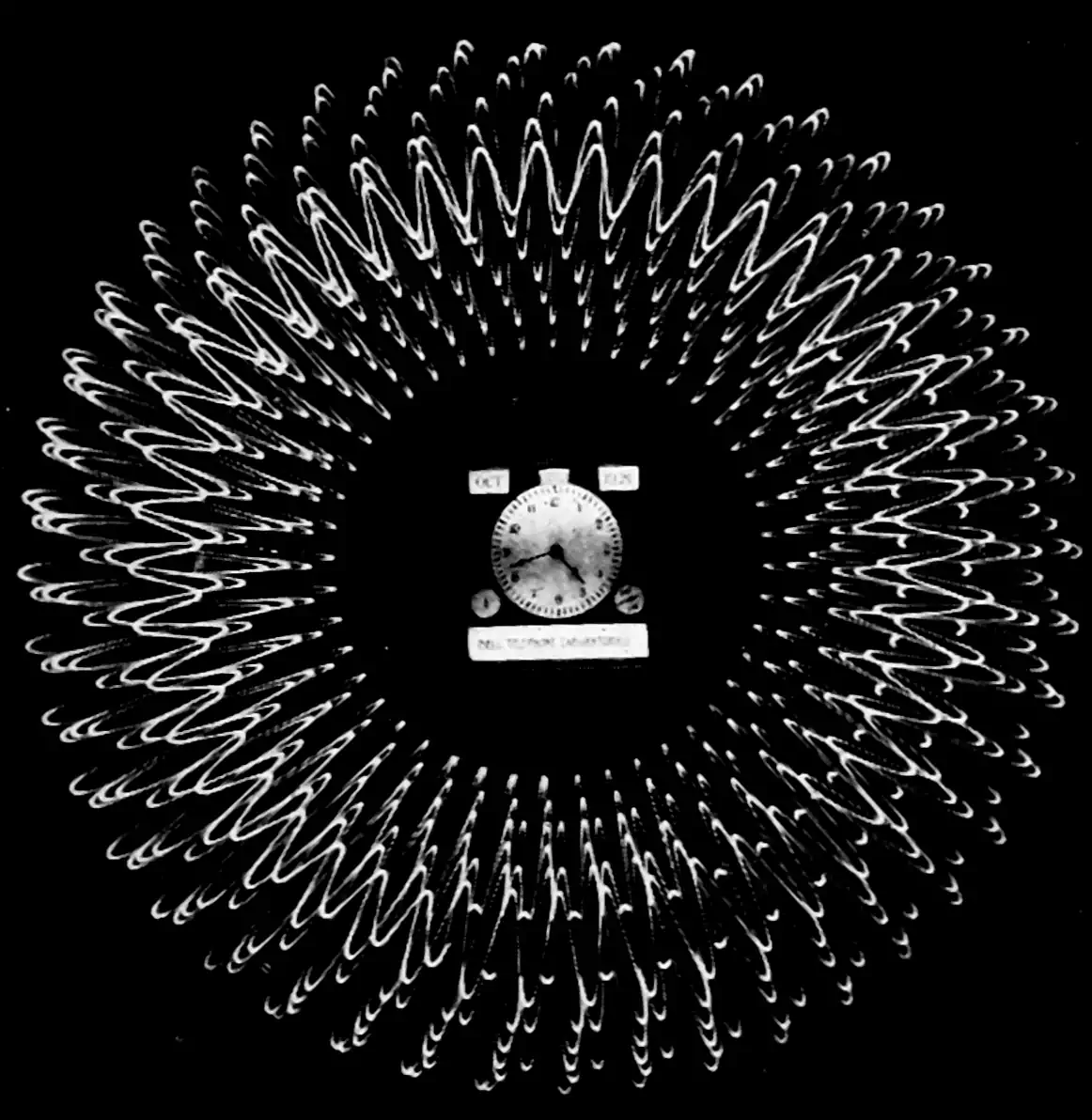
Correlograms

This material is revised and expanded from the appendix of draft versions of a recent conference submission, for my own reference. I used (deterministic) correlograms a lot in that, and it was startlingly hard to find a decent summary of their properties anywhere. Nothing new here, but… see the matrial about doing this in a probabilistic way via Wiener-Khintchine representation and covariance kernels which lead to a natural probabilistic spectral analysis.

\[\renewcommand{\var}{\operatorname{Var}} \renewcommand{\dd}{\mathrm{d}} \renewcommand{\pd}{\partial} \renewcommand{\bb}[1]{\mathbb{#1}} \renewcommand{\vv}[1]{\boldsymbol{#1}} \renewcommand{\mm}[1]{\mathrm{#1}} \renewcommand{\mmm}[1]{\mathrm{#1}} \renewcommand{\cc}[1]{\mathcal{#1}} \renewcommand{\ff}[1]{\mathfrak{#1}} \renewcommand{\oo}[1]{\operatorname{#1}} \renewcommand{\gvn}{\mid} \renewcommand{\II}[1]{\mathbb{I}\{#1\}} \renewcommand{\inner}[2]{\langle #1,#2\rangle} \renewcommand{\Inner}[2]{\left\langle #1,#2\right\rangle} \renewcommand{\finner}[3]{\langle #1,#2;#3\rangle} \renewcommand{\FInner}[3]{\left\langle #1,#2;#3\right\rangle} \renewcommand{\dinner}[2]{[ #1,#2]} \renewcommand{\DInner}[2]{\left[ #1,#2\right]} \renewcommand{\norm}[1]{\| #1\|} \renewcommand{\Norm}[1]{\left\| #1\right\|} \renewcommand{\fnorm}[2]{\| #1;#2\|} \renewcommand{\FNorm}[2]{\left\| #1;#2\right\|} \renewcommand{\argmax}{\operatorname{arg max}} \renewcommand{\argmin}{\operatorname{arg min}} \renewcommand{\omp}{\mathop{\mathrm{OMP}}}\]

Consider an \(L_2\) signal \(f: \bb{R}\to\bb{R}.\) We frequently overload notation and refer to as signal with free argument \(t\), so that \(f(rt-\xi),\) for example, refers to the signal \(t\mapsto f(rt-\xi).\) We write the inner product between signals \(t\mapsto f(t)\) and \(t\mapsto f'(t)\) as \(\inner{f(t)}{f'(t)}\). Where it is not clear that the free argument is, e.g. \(t\), we annotate it \(\finner{f(t)}{f'(t)}{t}\).

The correlogram \(\cc{A}:L_2(\bb{R}) \to L_2(\bb{R})\) maps signals to signals. Specifically, \(\mathcal{A}\{f\}\) is a signal \(\bb{R}\to\bb{R}\) such that

\[\mathcal{A}\{f\}:=\xi \mapsto \finner{ f(t) }{ f(t-\xi) }{t}\] This is the covariance between \(f(t)\) and \(f(t-\xi).\) (Note that we here discuss the covariance between given deterministic signals, not between two stochastic sources; covariance of stochastic processes is a broader, let alone inferring the covariance of stochastic processes.) Note also that this is what I would call an autocovariance not an auto-correlation, since it’s not normalized, but I’ll stick with the latter for now since for reasons of convention.

We derive the properties of this transform.

Multiplication by a constant. Consider a constant \(c\in \bb{R}.\)

\[\begin{aligned}\mathcal{A}\{cf\}(\xi)&= \inner{ cf(t) }{ cf(t-\xi) }\\ &= c^2\finner{ f(t) }{ f(t-\xi) }{t}\\ &= c^2\mathcal{A}\{f\}(\xi).\\ \end{aligned}\]

Time scaling:

\[\begin{aligned}\mathcal{A}\{f(r t)\}(\xi) &=\finner{ f(r t) }{ f(r t-\xi) }{t}\\ &= \int f(r t)f(r t-\xi)\dd t\\ &= \frac{1}{r }\int f(t)f(t-\frac{\xi}{r})\dd t\\ &= \frac{1}{r} \mathcal{A}\{f\}\left(\frac{\xi}{r}\right)\\ \end{aligned}\]

Addition:

\[\begin{aligned}\mathcal{A}\{f+f'\}(\xi) &=\finner{ f(t)+f'(t) }{ f(t-\xi)+f'(t-\xi) }{t}\\ &=\finner{ f(t) }{ f(t-\xi)\rangle+\langle f(t),f'(t-\xi) }{t} +\finner{ f'(t) }{ f(t-\xi)\rangle+\langle f'(t),f'(t-\xi) }{t}\\ &= \mathcal{A}\{f\}(\xi)+ \finner{ f'(t) }{ f(t-\xi)}{t} +\finner{f(t)}{f'(t-\xi) }{t} +\mathcal{A}\{f'\}(\xi).\\ &= \mathcal{A}\{f\}(\xi)+ \finner{ f'(t) }{ f(t-\xi)}{t} +\finner{f(t+\xi)}{f'(t) }{t} +\mathcal{A}\{f'\}(\xi).\\ &= \mathcal{A}\{f\}(\xi)+ \finner{ f'(t) }{ f(t-\xi)}{t} +\finner{f'(t) }{f(t+\xi)}{t} +\mathcal{A}\{f'\}(\xi).\\ \end{aligned}\]

We can say little about the term \(\finner{ f'(t) }{ f(t-\xi)}+\finner{f'(t) }{f(t+\xi)}{t}\) without more information about the signals in question. However, we can solve a randomized version. Suppose \(S_i, \, i \in\bb{N}\) are i.i.d. Rademacher variables, i.e. that they assume a value in \(\{+1,-1\}\) with equal probability. Then, we can introduce the following property:

Randomised addition:

\[\begin{aligned} \bb{E}[ \mathcal{A}\{S_1f + S_2f'\}(\xi) &=\bb{E}[ \mathcal{A}\{S_1f\}(\xi) + \finner{ S_2 f'(t) }{ S_1 f(t-\xi)}{t} +\finner{S_2f'(t) }{S_1 f(t+\xi)}{t} +\mathcal{A}\{S_2f'\}(\xi)]\\ &=\bb{E}[ \mathcal{A}\{S_1f\}(\xi)] + \bb{E}\finner{ S_2 f'(t) }{ S_1 f(t-\xi)}{t} + \bb{E}\finner{S_2f'(t) }{S_1 f(t+\xi)}{t} +\bb{E}[ \mathcal{A}\{S_2f'\}(\xi)]\\ &=\mathcal{A}\{f\}(\xi)+ \bb{E}[ S_1S_2]\finner{ f'(t) }{ f(t-\xi) }{t} + \bb{E}[ S_1S_2]\finner{ f'(t) }{ f(t+\xi) }{t}+\mathcal{A}\{f'\}(\xi)\\ &=\mathcal{A}\{f\}(\xi)+ \mathcal{A}\{f'\}(\xi)\\ \end{aligned}\]