Probabilistic graphical models
August 5, 2014 — February 8, 2022
The term graphical model in the context of statistics means a particular thing: a family of ways to relate inference in multivariate models in terms of Calculating marginal and conditional probabilities to graphs that describe how probabilities factorise, where graph here is in the sense of network theory, i.e. a collection of nodes connected by edges. Here are some of those ways:

It turns out that switching back and forth between these different formalisms makes some things easier to do and if you are luck also easier to understand. Within this area, there are several specialties and a lot of material. This is a landing page pointing to actual content.
Thematically, content to this theme is scattered across graphical models in variational inference, learning graphs from data, diagramming graphical models, learning causation from data plus graphs, quantum graphical models, and yet more pages.
1 Introductory texts
Barber (2012) and Lauritzen (1996) are rigorous introductions. Murphy (2012) presents a minimal introduction intermixed with particular related methods, so takes you straight to applications, although personally I found that confusing. For use in causality, Pearl (2009) and Spirtes, Glymour, and Scheines (2001) are readable.
People recommend me Koller and Friedman (2009) which is probably the most comprehensive, but I found it too comprehensive, to the point it was hard to see the forest for the trees. Maybe better as thing to deepen your understanding when you already know what is going on.
The insight of factor graphs is that we can turn this ⬆ problem into that ⬇ problem.
2 Basic inference
Dejan Vukobratovic: Gaussian Belief Propagation: From Theory to Applications is where I learnt the “Query”, “hidden” and “evidence” variables” terminology, without which we might wonder why anyone bothers doing anything with graphical models
3 What are plates?
Invented in Buntine (1994), the plate notation is how we introduce the notion of multiple variables with a regular, i.e. conditionally independent relation to existing variables. These are extremely important if you want to observe more than one data point. AFAICT, really digging deep into data as just another node is what makes Koller and Friedman (2009) a classic text book. But it is really glossed over in lots of papers, especially early ones, where the problem of estimating parameters from data is glossed over.
Concretely, consider Dustin Tran’s example of the kind of dimensionality we are working with:
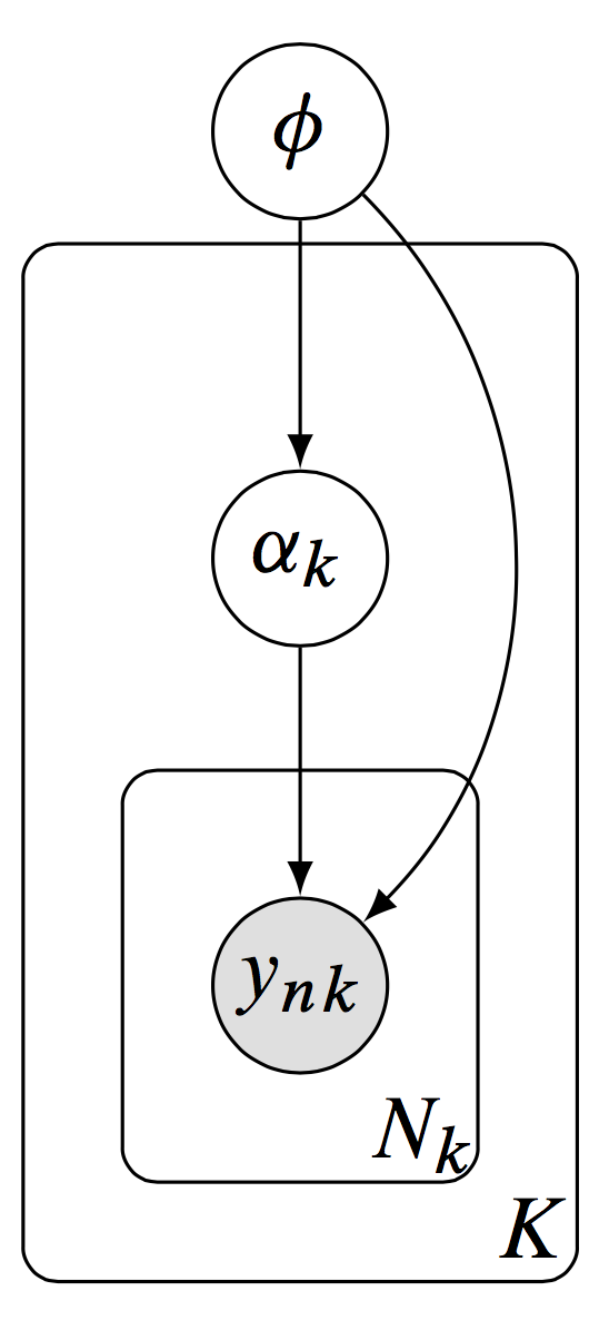
Dustin Tran: A hierarchical model, with latent variables \(\alpha_k\) defined locally per group and latent variables \(\phi\) defined globally to be shared across groups.
We are motivated by hierarchical models[…]. Formally, let \(y_{n k}\) be the \(n^{t h}\) data point in group \(k\), with a total of \(N_{k}\) data points in group \(k\) and \(K\) many groups. We model the data using local latent variables \(\alpha_{k}\) associated to a group \(k\), and using global latent variables \(\phi\) which are shared across groups.[…] (Figure) The posterior distribution of local variables \(\alpha_{k}\) and global variables \(\phi\) is \[ p(\alpha, \phi \mid \mathbf{y}) \propto p(\phi \mid \mathbf{y}) \prod_{k=1}^{K}\left[p\left(\alpha_{k} \mid \beta\right) \prod_{n=1}^{N_{K}} p\left(y_{n k} \mid \alpha_{k}, \phi\right)\right] \] The benefit of distributed updates over the independent factors is immediate. For example, suppose the data consists of 1,000 data points per group (with 5,000 groups); we model it with 2 latent variables per group and 20 global latent variables.
How many dimensions are we integrating over now? 10,020. The number of intermediate dimensions in our data grows very rapidly as we add observations, even if the final marginal is of low dimension. However, some of those dimensions are independent of others, and so may be factored away.
4 Directed graphs
Graphs of conditional, directed independence are a convenient formalism for many models. These are also called Bayes nets presumably because the relationships encoded in these graphs have utility in the automatic application of Bayes rule. These models have a natural interpretation in terms of causation and structural models. See directed graphical models.
5 Undirected, a.k.a. Markov graphs
a.k.a Markov random fields, Markov random networks… These have a natural interpretation in terms of energy-based models. See undirected graphical models.
6 Factor graphs
A unifying formalism for the directed and undirected graphical models. Simpler in some ways, harder in others. See factor graphs.
7 Inference on
A key use of this graphical structure is that it can make inference local, in that you can have different compute nodes, which examine part of the data/part of the model and pass messages back and forth to do inference over the entire thing. It is easy to say this, but making practical and performant algorithms this way is… well, it is a whole field. See graphical models in inference,
8 Implementations
All of the probabilistic programming languages end up needing to account for graphical model structure in practice, so maybe start there.